LSR-1

Seebeck coefficient & specific resistance

Description

To the point

With the Linseis LSR platform, thermoelectric materials in the form of bulk materials and thin films can be characterized in a simple and convenient way.
In the basic version – LSR-1 – both the Seebeck coefficient and the electrical resistance can be measured fully automatically and simultaneously from -160°C to 200°C.

The basic version of the LSR-1 (RT to 200°C) can be combined with various options to extend the application range.
For example, the low temperature option enables fully automatic measurements with LN2 cooling down to -160°C and quench cooling down to 80 K (resistance only).
An optional high-temperature probe stage enables resistance measurements up to 600°C.
With the illumination option, it is possible to carry out thermoelectric measurements under the defined influence of light, using a 3-wavelength LED light source.

The LSR-1 system enables the characterization of metallic and semiconducting samples using the well-known Van der Pauw (resistance), static direct current and slope Seebeck coefficient measurement techniques.

The compact table-top design enables fully automatic and software-controlled operation.
The comprehensive Windows-based software offers an easy-to-use user interface, including wizards for creating a measurement profile, feedback on the reliability of the measurement data and integrated measurement data evaluation and storage.
The vacuum-tight measuring chamber in combination with a choice of gas dosing systems ensures that all application areas can be covered.

Principle of measuring the Seebeck coefficient

  • The sample temperature and the temperature gradient are controlled by a heater embedded in the sample holder.
  • The temperature can be cooled down to approx. -160°C so that the specific resistance can be measured down to -160°C.
  • The Seebeck coefficient can be measured up to an average sample temperature of 180°C.
  • Increased precision in temperature measurement: The individual TC wires contact the sample surface orthogonally to the direction of the temperature gradient.
    Both contact points have the same temperature.
    This method measures the surface temperature of the sample and not the temperature of a TC bead pressed onto the sample surface.
    In this way, it is also irrelevant whether the temperature of the sample surface is affected by the TC wires transferring heat to/from the sample.
  • Improved precision thermoelectric voltage measurement: The Seebeck voltage is measured between the two negative TC wires, which enables the most accurate spatial correlation between temperature and thermoelectric voltage measurement.
    This means that the Seebeck voltage occurs exactly at the points where the temperature is also measured.
  • The Seebeck voltage is recorded together with the temperature gradient while the power of the gradient heater is increased linearly.
    The duration of a single measurement run is approximately 30 to 90 seconds, including the high-speed sampling rate.
    The values are sampled once per second.
  • The gradient of the thermoelectric voltage over delta T is adjusted with a linear polynomial regression.
    Thanks to this dynamic evaluation method, any offsets that occur during the temperature gradient measurement can be neglected and the measurement accuracy is increased.
    Due to the short duration of the actual measurement, offset drifts have very little influence on the result.

Principle of resistance measurement

The Van der Pauw measurement technique is used to determine the specific electrical resistance (or electrical conductivity) of the sample.
This allows samples of any shape to be analyzed, interfering influences such as contact or wire resistance are suppressed and the measurement accuracy can be significantly increased.

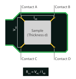
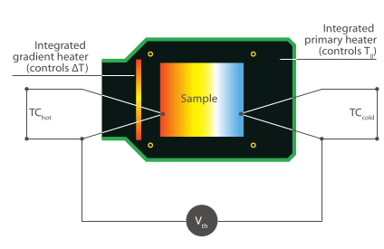
For the Van der Pauw measurement, the sample must be connected to four electrodes directly at the edge.
In the first step of the routing, a current is made to flow at two contacts on one edge of the sample and the voltage is measured at the other two contacts on the opposite edge.
A resistance can be determined from these two values using Ohm’s law.
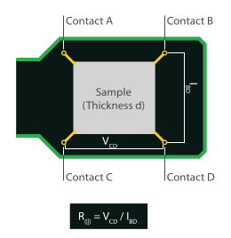
In the second step, the contacts are switched cyclically and the measurement is repeated.
The sheet resistance of the sample can then be easily calculated by substituting the two measured resistances (horizontal and vertical) into the Van der Pauw formula and solving.

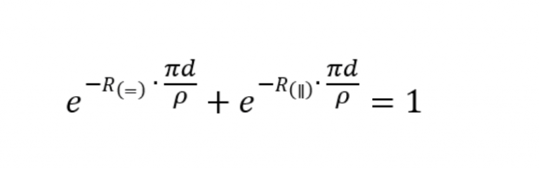
Based on the measured data and the thermocouple spacing “t”, the specific resistance and electrical conductivity can be calculated using the following formulae:

Unique features

Modular system design, can be
upgraded with gas purging system,
lighting and cryogenic option

Vacuum-tight measuring
chamber for measurements
under defined atmospheres

Interchangeable sample carriers with
integrated primary and secondary
heating and simple contact mechanism

Simultaneous measurement
of the Seebeck coefficient
and theelectrical resistance
(resistance)

Fully automatic, software-controlled measurements with
export options for raw data in various formats

Service hotline

+01 (609) 223 2070


+49 (0) 9287/880 0

Our service is available Monday to
Thursday from 8 am to 4 pm
and Friday from 8 am to 12 pm.

We are here for you!

Specifications

Black on white

Special features

  • Modular system design.
    Can be upgraded with gas purging system, lighting and cryogenic option.
  • Vacuum-tight measuring chamber for measurements under defined atmospheres.
  • Easy-to-use and interchangeable sample carriers with integrated primary and secondary heating.
  • Integrated state-of-the-art measurement technology for the most accurate results with demanding samples.
  • The unit can be used for simultaneous measurement of both the Seebeck coefficient and the electrical resistance (resistivity).
  • The sample carrier uses a special contact mechanism for easy sample preparation and enables measurements with high reproducibility.
  • V-I characteristic measurement can be performed to determine if the sensor has good contact with the sample.
  • The system enables fully automatic, software-controlled measurements with predefined temperature and measurement profiles.
  • The measured raw data is stored on the hard disk and can be exported in several data formats for further processing in Microsoft Excel or Origin.
  • The system is supplied with Constantan reference including tables and certificate.

MODEL

LSR-1

Temperature range:Basic unit: RT to 200°C
Cryo option: -160°C to +200°C
Principles of measurement:Seebeck coefficient measuring range: 0 to 2.5 mV/K - temperature gradient up to 10K
Seebeck voltage measurement: range +-8 mV
Atmospheres:Inert, reducing, oxidising, vacuum
Helium gas with low pressure, recommended
Sample holder:Integrated PCB board with primary and secondary heater
Sample size (Seebeck):L: 8 mm to 25 mm; W: 2 mm to 25 mm; D: Thin film up to 2 mm
Sample size (resistance):L: 18 mm to 25 mm; W: 18 mm to 25 mm; D: thin film up to 2 mm
Vacuum pump:optional
Heating rate:0.01 – 100 K/min
Temperature accuracy:±1,5 °C oder 0,0040 ∙ | t |
Electrical resistance:10 nOhm
Thermal voltage:0.5 nV/K (nV = 10-9 V)

Data sheet

Software

Making values visible and comparable

The powerful LINSEIS thermal analysis software, which is based on Microsoft® Windows®, performs the most important function in the preparation, execution and evaluation of thermoanalytical experiments alongside the hardware used.
With this software package, Linseis offers a comprehensive solution for programming all device-specific settings and control functions as well as for data storage and evaluation.
The package was developed by our in-house software specialists and application experts and has proven itself over many years.

General properties

  • Automatic evaluation of the Seebeck coefficient and electrical conductivity
  • Automatic control of sample contacting
  • Creation of automatic measurement programs
  • Creation of temperature profiles and temperature gradients for the Seebeck measurement
  • Color reproduction in real time
  • Automatic and manual scaling
  • Freely selectable display of the axes (e.g. temperature (x-axis) versus delta L (y-axis))
  • Mathematical calculations (e.g. first and second derivatives)
  • Database for archiving all measurements and evaluations
  • Multitasking (different programs can be used simultaneously)
  • Multi-user option (user accounts)
  • Zoom options for curve sections
  • Any number of curves can be loaded on top of each other for comparison
  • Menu online help
  • Free labeling of curves
  • Simplified export functions (CTRL C)
  • EXCEL® and ASCII export of measurement data
  • Statistical trend analysis (mean value curve with confidence interval)
  • Tabular presentation of the data

Applications

Application example: Evaluation of acquired data using linear regression

Seebeck voltage/temperature gradient (blue), measured during the sweep of the gradient heating power together with the linear regression (red).
The Seebeck coefficient is determined by the slope of the linear regression.

Application example: Data evaluation

In this method, the Seebeck coefficient is measured relative to Alumel.
To calculate the absolute Seebeck coefficient, platinum is measured relative to the Alumel wire via the temperature.

Application example: Seebeck coefficient compared to temperature

Example for the measurement of the Seebeck coefficient of constantan.

Videos

Well informed

Downloads

Everything at a glance